A top 10 list is a common form for displaying information, especially on dashboards and summarized reports. It is easy to create the list when working with sorted data, just cell link to the top 10 items in the list… easy! It’s also relatively simple when using Auto Filter, Tables and Pivot Tables, as it is a default filter setting within these features. However, when creating a top 10 with formulas on a non-sorted dataset, things become a little bit tricky. In this post, I will show you exactly how to do it. Through these methods, you’re not restricted to a top 10; you can create a top 5, top 8, or any number you choose.
Some of the most common formula problems with top 10 lists are:
- Dealing with duplicate values
- Working with categories
- How to change it to get the bottom 10
Don’t worry, we will cover all of these (they are also all included in the example file). Hopefully, along the way, you’ll learn a little more about how Excel works.
Dynamic arrays
Users with an Office 365 subscription now have access to a group of functions, which make use of the new dynamic array calculation engine. These give us a nice simple way to calculate a top 10. So, if you have a dynamic array enabled version of Excel, then be sure to check out that section.
Download the example file
I recommend you download the example file for this post. Then you’ll be able to work along with examples and see the solution in action, plus the file will be useful for future reference.
Download the file: 0015 Top 10 using formulas.zip
Note: If you don’t have a Dynamic Array enabled version of Excel, the tabs containing those examples will display errors.
Watch the video:
Contents
Traditional functions
We are going to start with traditional functions (i.e., non-dynamic array). Using these, it is easy to obtain the top 10 values. But getting the names/labels which relate to those ten values is the challenge.
Start by looking at the Top 10 – non-DA tab of the example file.
Using the LARGE function
In our example file, there are 26 customers, with their values.
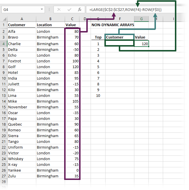
If we wanted to create a top 10 of these customers (without sorting the list), we could use the LARGE function. Cell G4 contains this formula:
=LARGE($C$2:$C$27,ROW(F4)-ROW(F$3))
LARGE only has two arguments:
=LARGE(Range, k)
- Range – The range of data to be analyzed.
- k – The nth item to be found.
In our example, the data range to analyze is cells C2 to C27.
The k value is calculated as the row number, minus the row number of the header row. This always calculates the relative row position in a range of cells. The first row of data calculates as 1, the second row, calculates as 2, and so on.
ROW(F4)-ROW(F$3)
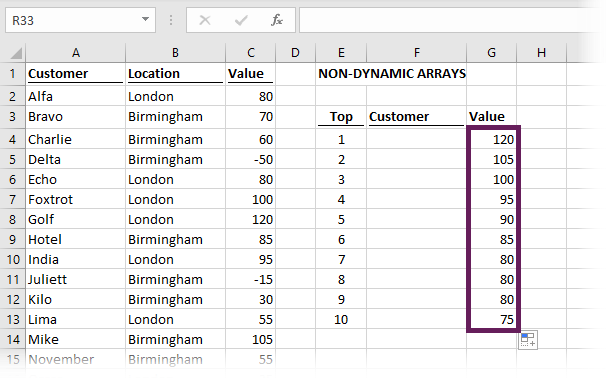
The formula in cell G4 has been copied down to display the top 10 values.
Finding the labels for the top 10
We have the values, so now we can calculate the customer name for that value.
We can’t use VLOOKUP as the customer name is to the left of the lookup value. Instead, we will use the INDEX/MATCH formula combination. Cell F4, in our example, would contain the following formula.
=INDEX($A$2:$A$27,MATCH(G4,$C$2:$C$27,0))
If this formula were copied down into cells F5 – F13. Our worksheet would display as follows:
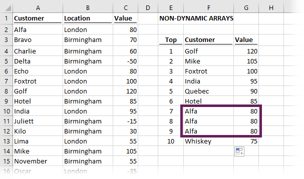
There is one huge problem – our top 10 values are not unique; there are 3 values of 80 (see the screenshot above). A basic INDEX/MATCH only returns the first value, so it finds the name Alfa 3 times. Yet, Echo and Tango, who also have 80, do not feature on the list. This is clearly an error, so how do we get around this?
Finding the labels when the top 10 values are not unique
To solve the issue of finding labels with non-unique values, we will turn to an advanced array formula. The formula in cell F4 should be:
{=INDEX($A$2:$A$27,SMALL(IF($C$2:$C$27=G4,ROW($C$2:$C$27)-ROW($C$1)),
COUNTIF($G$4:G4,G4)))}
Woah!!! That’s big and complicated!.
This is a special type of formula, known as an array formula. Don’t put the curly brackets ( { } ) at the start or the end when typing the formula into the formula bar; when you press Ctrl+Shift+Enter, Excel will add these itself. Pressing Ctrl+Shift+Enter lets Excel know that it is an array formula.REMEMBER! – If you go back into an array formula to edit it, you need to press Ctrl + Shift + Enter again to re-enter the formula.
This formula is like INDEX/MATCH, but returns the 1st, 2nd, 3rd, 4th… or nth value. Let’s dig a bit deeper to understand how it works.
Section 1 – IF function
In the middle of the formula, we find an IF function.
IF($C$2:$C$27=G4,ROW($C$2:$C$27)-ROW($C$1))
In English, this says:
If C2 = G4 then return the count of rows between C2 and C1.
As this is an array formula, it automatically goes onto the next row and calculates again
If C3 = G4 then return the count of rows between C3 and C1.
And it keeps on going
If C4 = G4 then return the count of rows between C4 and C1.
This will go all the way from C2 to C27.
For the formula in F4, the IF function calculates as:
{FALSE;FALSE;FALSE;FALSE;FALSE;FALSE;7;FALSE;FALSE;FALSE;FALSE;FALSE;FALSE;
FALSE;FALSE;FALSE;FALSE;FALSE;FALSE;FALSE;FALSE;FALSE;FALSE;FALSE;FALSE;FALSE}
The 7th item in the list matches cell G4; therefore, the only value which is not FALSE is 7.
Section 2 – SMALL and COUNTIF functions
If we feed this into the SMALL function, it would be as follows:
SMALL({FALSE;FALSE;FALSE;FALSE;FALSE;FALSE;7;FALSE;FALSE;FALSE;FALSE;FALSE;FALSE;
FALSE;FALSE;FALSE;FALSE;FALSE;FALSE;FALSE;FALSE;FALSE;FALSE;FALSE;FALSE;FALSE},
COUNTIF($G$4:G4,G4))
SMALL finds the nth smallest value. It works in a similar way to LARGE, but for the smallest value.
SMALL only has two arguments:
=SMALL(Range,k)
- Range – The range of data to be analyzed.
- k – The nth item to be found.
In this context, COUNTIF calculates how many instances of the value have appeared in the top 10 already.
For the first row, there is only 1 item in the top 10 with a score of 120, so COUNTIF will calculate as 1.
The SMALL will find the first smallest value, which is 7, as all the other results are FALSE.
Finally, let’s wrap that in the INDEX function to find the 7th value in the source table.
=INDEX($A$2:$A$27,7)
This calculates to cell A8, which in our example is Golf.
All the workings above were to show how the formula works. Now we can copy the complete formula down into cells F5 – F13.
Testing on duplicate values
The first row does not have a duplicate value. So, let’s test it out with cell F11. There are 3 values in the top 10 which are all 80; they are found in G10, G11 and G12. The label in F11 should be Echo, as it is the 2nd value of 80.
The formula in F11 is:
{=INDEX($A$2:$A$27,SMALL(IF($C$2:$C$27=G11,ROW($C$2:$C$27)-ROW($C$1)),
COUNTIF($G$4:G11,G11)))}
The IF portion of the function calculates as:
{1;FALSE;FALSE;FALSE;5;FALSE;FALSE;FALSE;FALSE;FALSE;FALSE;FALSE;FALSE;
FALSE;FALSE;FALSE;FALSE;FALSE;FALSE;20;FALSE;FALSE;FALSE;FALSE;FALSE;FALSE}
Rows 1, 5, and 20 in the source table all match the value of 80.
The COUNTIF calculates to 2, which makes sense, as it is the 2nd matching value we are looking for.
SMALL({1;FALSE;FALSE;FALSE;5;FALSE;FALSE;FALSE;FALSE;FALSE;FALSE;FALSE;FALSE;
FALSE;FALSE;FALSE;FALSE;FALSE;FALSE;20;FALSE;FALSE;FALSE;FALSE;FALSE;FALSE},2)
As the second smallest number is 5, the INDEX function returns the 5th value in the source list, which is Echo.
Fantastic stuff, right!!!
Bottom 10 values
If you want the bottom 10 values, the only change is that the formula to get the values uses SMALL, rather than LARGE.
Look at the example file. The formula in cell G18 is:
=SMALL($C$2:$C$27,ROW(F18)-ROW($F$17))
The only difference between cell G18 and cell G4 is the use of the SMALL function.
The formula in cell F18 is the same as we saw above before (but pointing at different cells).
=INDEX($A$2:$A$27,SMALL(IF($C$2:$C$27=G18,ROW($C$2:$C$27)-ROW($C$1)),
COUNTIF($G$18:G18,G18)))
Adding criteria
Sometimes we want to calculate the top 10 results where a specific condition is met. In our example file, look at the Top 10 – non-DA with criteria tab.
Cell J4 contains the name of the city; London or Birmingham. The top 10 will only be returned for customers in that city.
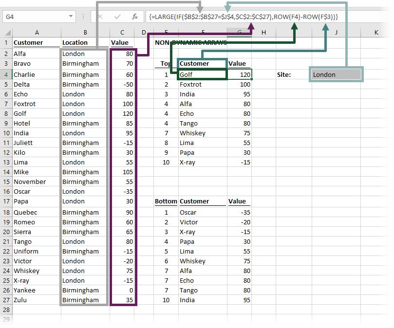
Cell G4 has the following function:
{=LARGE(IF($B$2:$B$27=$J$4,$C$2:$C$27),ROW(F4)-ROW(F$3))}
This is another array formula. Remember, don’t enter the curly brackets, but do press Ctrl+Shift+Enter again.
This uses the same logic as we’ve already seen. The IF function checks cells B2 to B27; if the value matches cell J4, the value in C2 to C27 is returned.
When the city is London, the IF calculate as follows:
{80;FALSE;FALSE;FALSE;80;100;120;FALSE;95;FALSE;FALSE;55;FALSE;FALSE;
-35;30;FALSE;FALSE;FALSE;80;FALSE;-20;75;-15;FALSE;FALSE}
By using the LARGE function, only the London values will be returned into the top 10. All the non-London values calculate as FALSE.
We make a similar adjustment to the formula which calculates the customer name (the added section is in bold)
={INDEX($A$2:$A$27,SMALL(
IF(($C$2:$C$27=G4)*($B$2:$B$27=$J$4),ROW($C$2:$C$27)-ROW($C$1)),
COUNTIF(G4:$G$4,G4)))}
This is an array formula. Don’t enter the curly brackets. Do press Ctrl+Shift+Enter again.
This uses similar TRUE/FALSE logic to only calculate the values which match the city selected.
Look at the example file (Cells E17 – H27) if you want to see how a bottom 10 with criteria is calculated.
Generate accurate VBA code in seconds with AutoMacro
Dynamic array functions
Everything above seems quite complicated. Wouldn’t it be better if we could use some more straightforward formulas? If you have a dynamic array enabled version of Excel (only available to Office 365 subscribers at the time of writing), then you’re in luck.
INDEX / SORT / SEQUENCE function combination
Look at the Top 10 DA tab of the example file.
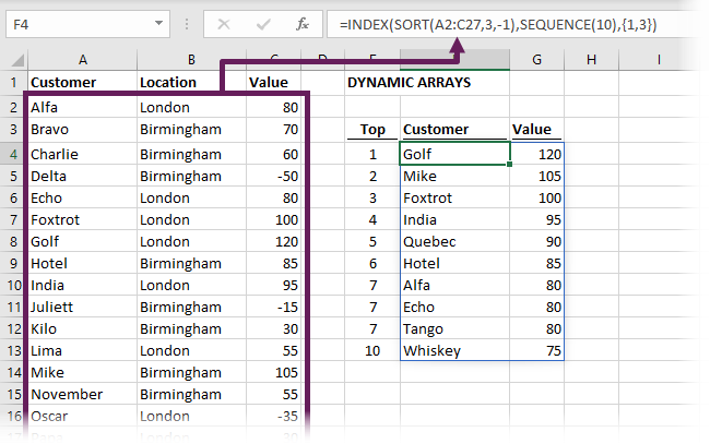
In cell F4 the formula is:
=INDEX(SORT(A2:C27,3,-1),SEQUENCE(10),{1,3})
And that’s it! No more array formulas required for the top 10, no need to press Ctrl+Shirt+Enter, no need to copy down.
Let’s dig into this a bit deeper.
SORT
SORT has four arguments:
=SORT(array, [sort_index], [sort_order], [by_col])
- array: The range of cells, or array of values to be sorted.
- [sort_index]: The nth column or row to apply the sort to. For example, to sort by the 3rd column, the sort index would be 3.
- [sort_order]: 1 = sort in ascending order, -1 = sort in descending order (if excluded the argument will default to 1).
- [by_col]: TRUE = sort by columns, FALSE = sort by rows (if excluded the argument will default to FALSE).
In our formula, we used the following SORT.
SORT(A2:C27,3,-1)
This sorts the cells A2 to C27 on the 3rd column in descending order.
SEQUENCE
The SEQUENCE function has four arguments:
=SEQUENCE(Rows, [Columns], [Start], [Step])
- Rows: The number of rows to return
- [Columns]: The number of columns to return. If excluded, it will return a single column.
- [Start]: The first number in the sequence. If omitted, it will start at 1.
- [Step]: The amount to increment each subsequent value. If excluded, each increment will be 1.
In our example, the following creates a list from 1 to 10. We only need the first argument, as we can use the default options for the optional arguments.
SEQUENCE(10)
INDEX
Let’s put both SORT and SEQUENCE into a traditional INDEX function:
=INDEX(SORT(A2:C27,3,-1),SEQUENCE(10),{1,3})
The formula returns the first 10 results from the SORT and returns columns 1 and 3.
That was so easy… right.
Bottom 10
To get the bottom 10, we only need to change the 3rd argument of the SORT function from -1 to 1. Look at cell F18 in the example file to see this in action.
report this adDynamic arrays with criteria
Even if we have criteria to apply, it is still straight forward with dynamic arrays.
Now, look at the Top 10 – DA with criteria tab in the example file.
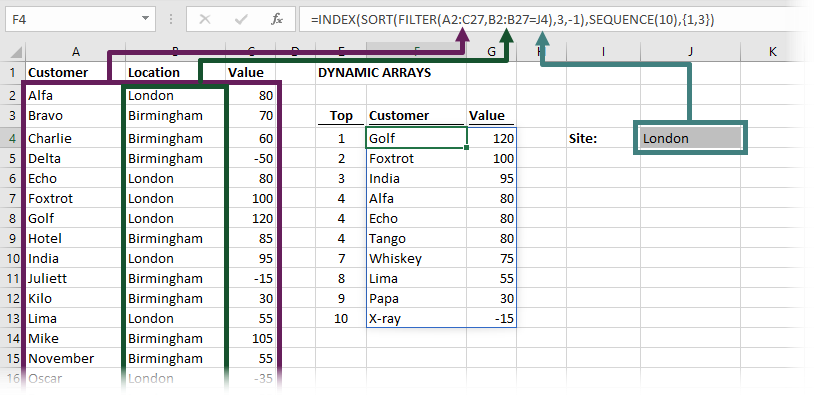
The formula in Cell F4 is:
=INDEX(SORT(FILTER(A2:C27,B2:B27=J4),3,-1),SEQUENCE(10),{1,3})
The only difference to the previous example is that we are using the FILTER function to only include the matching items, before it is fed into the SORT function.
FILTER
FILTER has three arguments:
=FILTER(array, include, [if_empty])
- array: The range of cells, or array of values to filter.
- include: An array of TRUE/FALSE results, where the TRUE values will be retained in the filter.
- [if_empty]: The value to display if no rows are returned.
In our example, the FILTER function is:
FILTER(A2:C27,B2:B27=J4)
It is returning cells A2 to C27, but only where the values from B2 to B27 equals the selected city in cell J4.
Conclusion
Once you know the techniques and the formulas, calculating a top 10 using formulas in Excel isn’t too bad.
This post demonstrates how good dynamic arrays are; we don’t need to rely on complex array formulas any longer.
Don’t forget:
If you’ve found this post useful, or if you have a better approach, then please leave a comment below.