How to Convert Number to Text or Reverse in Excel

You can use the VALUE function to return just the numeric value of the text.

1. Insert a new column

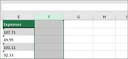
Insert a new column next to the cells with text. In this example, column E contains the text stored as numbers. Column F is the new column.

2. Use the VALUE function

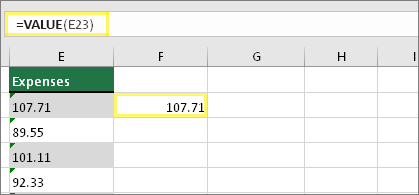
In one of the cells of the new column, type =VALUE() and inside the parentheses, type a cell reference that contains text stored as numbers. In this example it’s cell E23.

3. Rest your cursor here

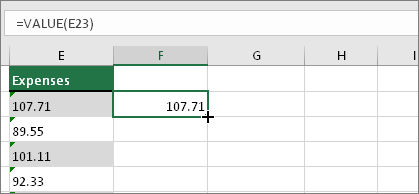
Now you’ll fill the cell’s formula down, into the other cells. If you’ve never done this before, here’s how to do it: Rest your cursor on the lower-right corner of the cell until it changes to a plus sign.

4. Click and drag down

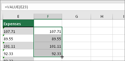
Click and drag down to fill the formula to the other cells. After that’s done, you can use this new column, or you can copy and paste these new values to the original column. Here’s how to do that: Select the cells with the new formula. Press CTRL + C. Click the first cell of the original column. Then on the Home tab, click the arrow below Paste, and then click Paste Special > Values.

Convert number to text

If you use Excel spreadsheets to store long and not so long numbers, one day you may need to convert them to text. There may be different reasons to change digits stored as numbers to text. Below you’ll find why you may need to make Excel see the entered digits as text, not as number.

• Search by part not by the entire number. For example, you may need to find all numbers that contain 50, like in 501, 1500, 1950, etc.)
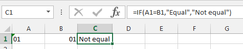
• It may be necessary to match two cells using the VLOOKUP or MATCH function. However, if these cells are formatted differently, Excel will not see identical values as matching. For instance, A1 is formatted as text and B1 is number with format 0. The leading zero in B2 is a custom format. When matching these 2 cells Excel will ignore the leading 0 and will not show the two cells as identical. That’s why their format should be unified.
  

The same issue can occur if the cells are formatted as ZIP code, SSN, telephone number, currency, etc.

In this article I’ll show you how to convert numbers to text with the help of the Excel TEXT function. If you are not so formula-oriented, have a look at the part where I explain how to change digits to text format with the help of the standard Excel Format Cells window, by adding an apostrophe and employing the Text to Columns wizard.

1. Convert number to text using the Excel TEXT function

The most powerful and flexible way to convert numbers to text is using the TEXT function. It turns a numeric value into text and allows to specify the way this value will be displayed. It’s helpful when you need to show numbers in a more readable format, or if you want to join digits with text or symbols. The TEXT function converts a numeric value to formatted text, thus the result cannot be calculated.

If you are familiar with using formulas in Excel, it will not be a problem for you to employ the TEXT function.

1. Add a helper column next to the column with the numbers to format. In my example, it’s column D.
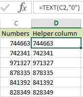
2. Enter the formula =TEXT(C2,"0") to the cell D2. In the formula, C2 is the address of the first cell with the numbers to convert.
3. Copy the formula across the column using the fill handle.
   
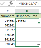
4. You will see the alignment change to left in the helper column after applying the formula.
   
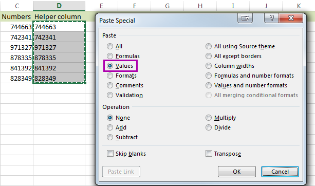
5. Now you need to convert formulas to values in the helper column. Start with selecting the column.
6. Use Ctrl + C to copy. Then press the Ctrl + Alt + V shortcut to display the Paste Special dialog box.
7. On the Paste Special dialog, select the Values radio button in the Paste group.
   You will see a tiny triangle appear in the top-left corner of each cell in your helper column, which means the entries are now text versions of the numbers in your main column.
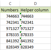   Now you can either rename the helper column and delete the original one, or copy the results to your main and remove the temporary column.Note. The second parameter in the Excel TEXT function shows how the number will be formatted before being converted. You may need to adjust this based on your numbers:The result of =TEXT(123.25,"0") will be 123.The result of =TEXT(123.25,"0.0") will be 123.3.The result of =TEXT(123.25,"0.00") will be 123.25.To keep the decimals only, use =TEXT(A2,"General").Tip. Say you need to format a cash amount, but the format isn’t available. For instance, you cannot display a number as British Pounds (£) as you use the built-in formatting in the English U.S. version of Excel. The TEXT function will help you convert this number to Pounds if you enter it like this: =TEXT(A12,"£#,###,###.##"). Just type the format to use in quotes -> insert the £ symbol by holding down Alt and pressing 0163 on the numeric keypad -> type #,###.## after the £ symbol to get commas to separate groups, and to use a period for the decimal point. The result is text!

2. Use the Format Cells option to convert number to text in Excel

If you need to quickly change the number to string, do it with the Format Cells… option.

1. Select the range with the numeric values you want to format as text.
2. Right click on them and pick the Format Cells… option from the menu list.
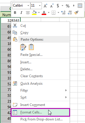   Tip. You can display the Format Cells… window by pressing the Ctrl + 1 shortcut.
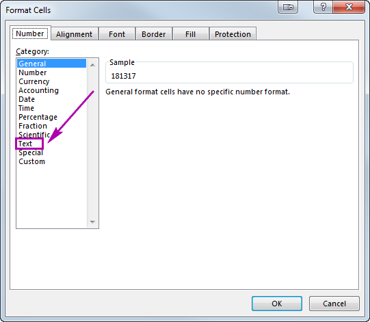
3. On the Format Cells window select Text under the Number tab and click OK.
   

You’ll see the alignment change to left, so the format will change to text. This option is good if you don’t need to adjust the way your numbers will be formatted.

3. Add an apostrophe to change number to text format

If these are just 2 or 3 cells in Excel where you want to convert numbers to string, benefit from adding an apostrophe before the number. This will instantly change the number format to text.

Just double-click in a cell and enter the apostrophe before the numeric value.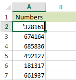

You will see a small triangle added in the corner of this cell. This is not the best way to convert numbers to text in bulk, but it’s the fastest one if you need to change just 2 or 3 cells.

4. Convert numbers to text in Excel with Text to Columns wizard

You may be surprised but the Excel Text to Columns option is quite good at converting numbers to text. Just follow the steps below to see how it works.

1. Select the column where you want to convert numbers to string in Excel.
2. Navigate to the Data tab in and click on the Text to Columns icon.
   
3. Just click through steps 1 and 2. On the third step of the wizard, make sure you select the Text radio button.
   
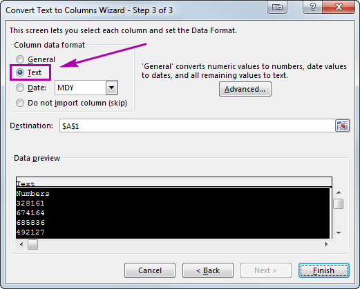
4. Press Finish to see your numbers immediately turn into text.

I hope the tips and tricks from this article will help you in your work with numeric values in Excel. Convert number to string using the Excel TEXT function to adjust the way your numbers will be displayed, or use Format Cells and Text to Columns for quick conversions in bulk. If these are just several cells, add an apostrophe. Feel free to leave your comments if you have anything to add or ask. Be happy and excel in Excel!

Ref: https://www.ablebits.com/office-addins-blog/2014/10/10/excel-convert-number-text/