Like VLOOKUP, the INDEX and MATCH functions pull in data from another dataset into one central location. Here are the main differences:
- VLOOKUP is a much simpler formula. If you’re working with large data sets that would require thousands of lookups, using the INDEX MATCH function will significantly decrease load time in Excel.
- INDEX MATCH formulas work right-to-left, whereas VLOOKUP formulas only work as a left-to-right lookup. In other words, if you need to do a lookup that has a lookup column to the right of the results column, then you’d have to rearrange those columns in order to do a VLOOKUP. This can be tedious with large datasets and/or lead to errors.
So if I want to combine information in Sheet 1 and Sheet 2 onto Sheet 1, but the column values in Sheets 1 and 2 aren’t the same, then to do a VLOOKUP, I would need to switch around my columns. In this case, I’d choose to do an INDEX MATCH instead.
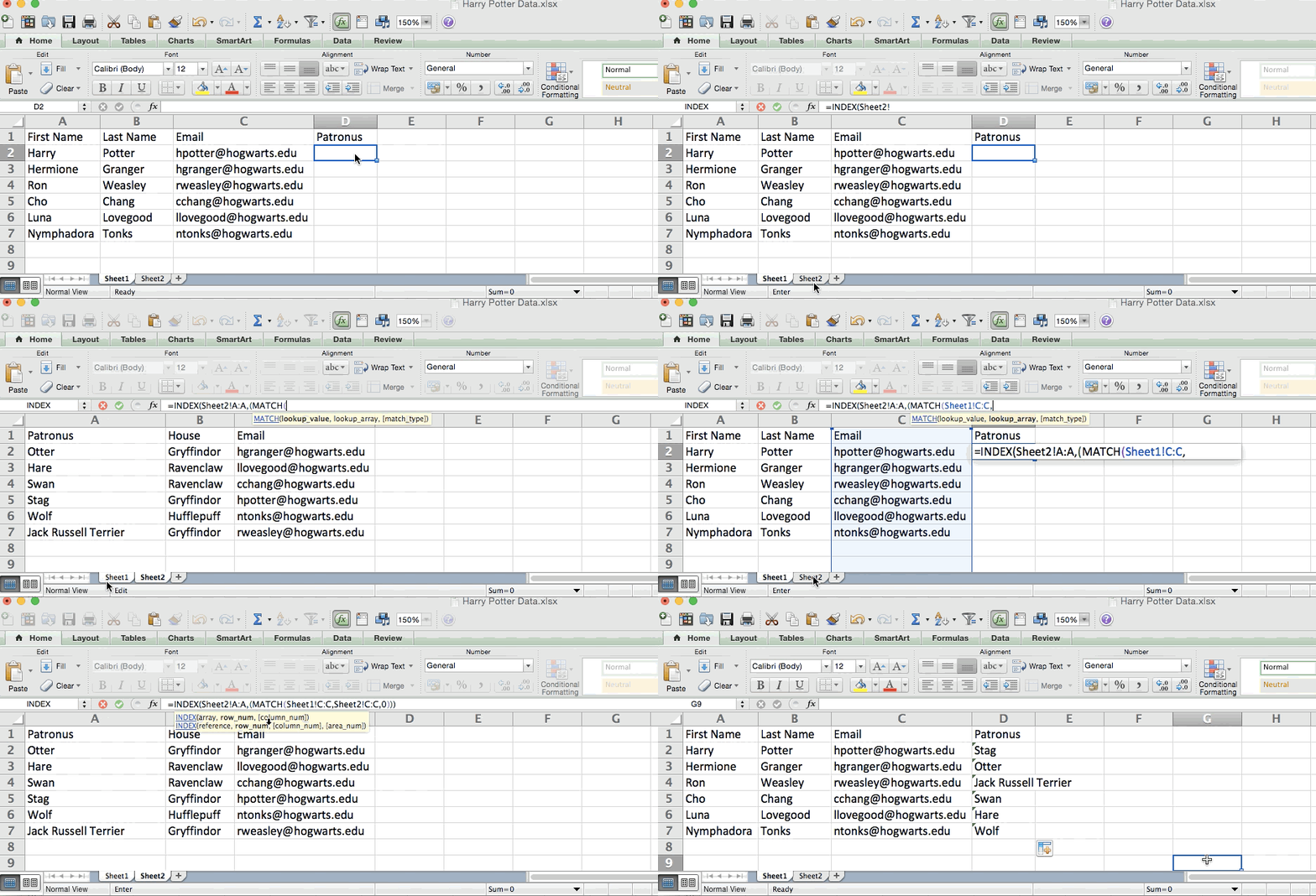
Let’s look at an example. Let’s say Sheet 1 contains a list of people’s names and their Hogwarts email addresses, and Sheet 2 contains a list of people’s email addresses and the Patronus that each student has. (For the non-Harry Potter fans out there, every witch or wizard has an animal guardian called a “Patronus” associated with him or her.) The information that lives in both sheets is the column containing email addresses, but this email address column is in different column numbers on each sheet. I’d use the INDEX MATCH formula instead of VLOOKUP so I wouldn’t have to switch any columns around.
So what’s the formula, then? The INDEX MATCH formula is actually the MATCH formula nested inside the INDEX formula. You’ll see I differentiated the MATCH formula using a different color here.
The formula: =INDEX(table array, MATCH formula)
This becomes: =INDEX(table array, MATCH (lookup_value, lookup_array))
The formula with variables from our example below: =INDEX(Sheet2!A:A,(MATCH(Sheet1!C:C,Sheet2!C:C,0)))
Here are the variables:
- Table Array: The range of columns on Sheet 2 containing the new data you want to bring over to Sheet 1. In our example, “A” means Column A, which contains the “Patronus” information for each person.
- Lookup Value: This is the column in Sheet 1 that contains identical values in both spreadsheets. In the example that follows, this means the “email” column on Sheet 1, which is Column C. So: Sheet1!C:C.
- Lookup Array: This is the column in Sheet 2 that contains identical values in both spreadsheets. In the example that follows, this refers to the “email” column on Sheet 2, which happens to also be Column C. So: Sheet2!C:C.
Once you have your variables straight, type in the INDEX MATCH formula in the top-most cell of the blank Patronus column on Sheet 1, where you want the combined information to live.

Ref: https://blog.hubspot.com/marketing/how-to-use-excel-tips