Have you ever had two sets of data on two different spreadsheets that you want to combine into a single spreadsheet?
For example, you might have a list of people’s names next to their email addresses in one spreadsheet, and a list of those same people’s email addresses next to their company names in the other — but you want the names, email addresses, and company names of those people to appear in one place.
I have to combine data sets like this a lot — and when I do, the VLOOKUP is my go-to formula. Before you use the formula, though, be absolutely sure that you have at least one column that appears identically in both places. Scour your data sets to make sure the column of data you’re using to combine your information is exactly the same, including no extra spaces.
The formula: =VLOOKUP(lookup value, table array, column number, [range lookup])
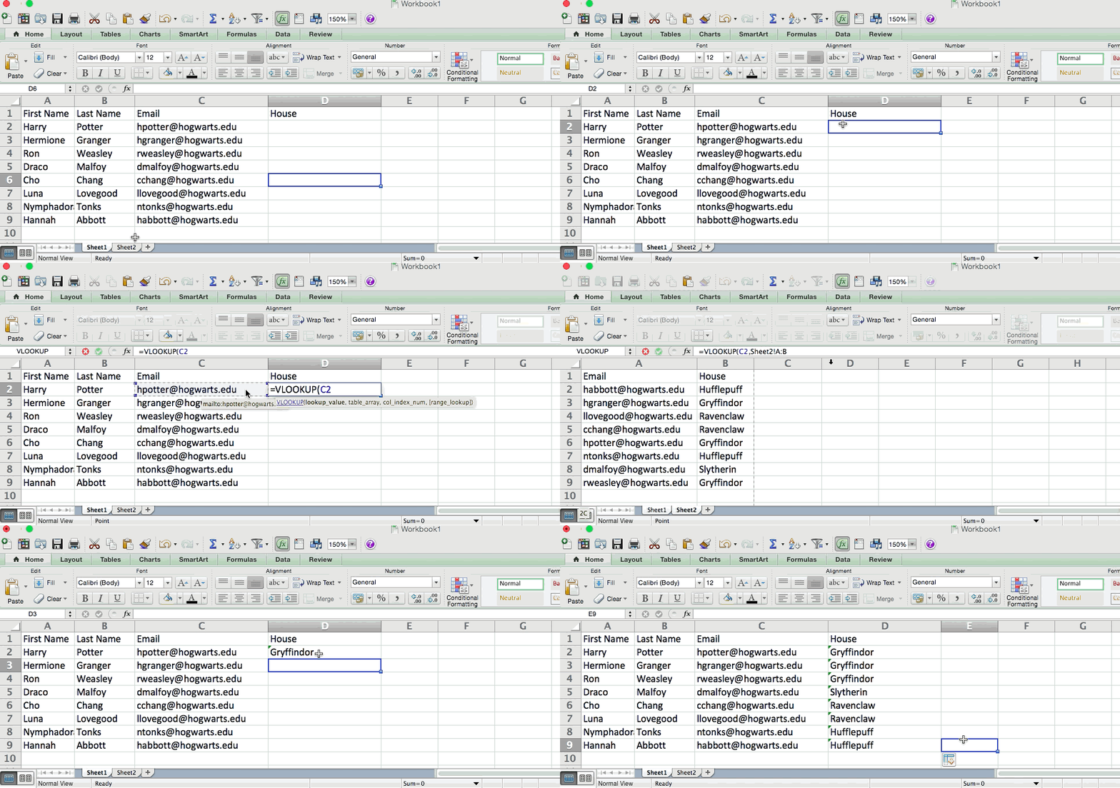
The formula with variables from our example below: =VLOOKUP(C2,Sheet2!A:B,2,FALSE)
In this formula, there are several variables. The following is true when you want to combine information in Sheet 1 and Sheet 2 onto Sheet 1.
- Lookup Value: This is the identical value you have in both spreadsheets. Choose the first value in your first spreadsheet. In the example that follows, this means the first email address on the list, or cell 2 (C2).
- Table Array: The range of columns on Sheet 2 you’re going to pull your data from, including the column of data identical to your lookup value (in our example, email addresses) in Sheet 1 as well as the column of data you’re trying to copy to Sheet 1. In our example, this is “Sheet2!A:B.” “A” means Column A in Sheet 2, which is the column in Sheet 2 where the data identical to our lookup value (email) in Sheet 1 is listed. The “B” means Column B, which contains the information that’s only available in Sheet 2 that you want to translate to Sheet 1.
- Column Number: If the table array (the range of columns you just indicated) this tells Excel which column the new data you want to copy to Sheet 1 is located in. In our example, this would be the column that “House” is located in. “House” is the second column in our range of columns (table array), so our column number is 2. [Note: Your range can be more than two columns. For example, if there are three columns on Sheet 2 — Email, Age, and House — and you still want to bring House onto Sheet 1, you can still use a VLOOKUP. You just need to change the “2” to a “3” so it pulls back the value in the third column: =VLOOKUP(C2:Sheet2!A:C,3,false).]
- Range Lookup: Use FALSE to ensure you pull in only exact value matches.
In the example below, Sheet 1 and Sheet 2 contain lists describing different information about the same people, and the common thread between the two is their email addresses. Let’s say we want to combine both datasets so that all the house information from Sheet 2 translates over to Sheet 1.

So when we type in the formula =VLOOKUP(C2,Sheet2!A:B,2,FALSE), we bring all the house data into Sheet 1.
Keep in mind that VLOOKUP will only pull back values from the second sheet that are to the right of the column containing your identical data. This can lead to some limitations, which is why some people prefer to use the INDEX and MATCH functions instead.
Ref: