This tutorial will guide you on how to make a checkbox in Excel and use the check box results in formulas to create an interactive checklist, to-do list, report or graph.
I believe everybody knows what a checkbox is, you must have seen plenty of them on various forms online. Still, for the sake of clarity, let me begin with a brief definition.
A check box, also referred to as a tick box or checkmark box or selection box, is a little square box where you click to select or deselect a given option.
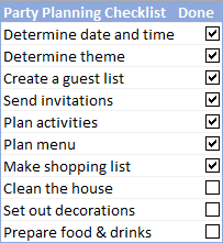
Inserting a checkbox in Excel sounds like a trivial thing, but it opens up a host of new possibilities for your worksheets that will keep you on track with your goals, schedule, assignments, etc.
- How to add checkbox in Excel
- How to use checkboxes in Excel – examples
- How to link a checkbox to a cell
- Make an Excel checklist
- Create a to-do list with conditional formatting
- Create an interactive report
- Make a dynamic chart
How to insert checkbox in Excel
Like all other Form controls, the Check Box control resides on the Developer tab, which does not appear on the Excel ribbon by default. So, you need to turn it on first.
1. Show the Developer tab on the ribbon
To add the Developer tab to the Excel ribbon, do the following:
- Right-click anywhere on the ribbon, and then click Customize the Ribbon… Or, click File > Options > Customize Ribbon.
- Under Customize the Ribbon, select Main Tabs (usually it is selected by default), check the Developer box, and click OK.
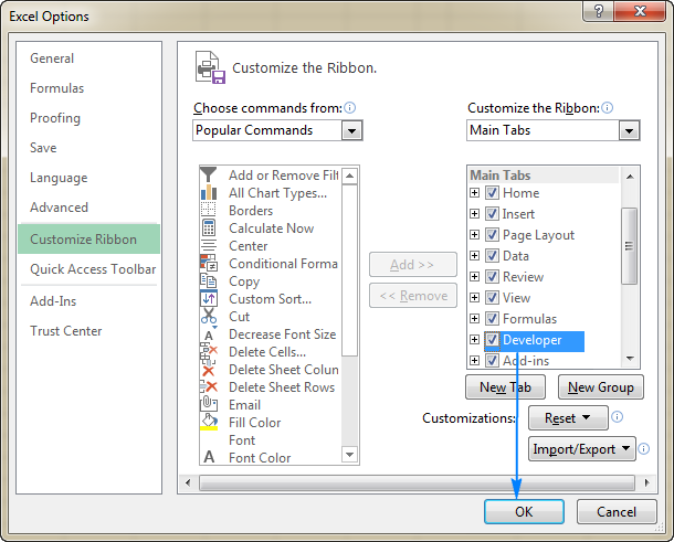
Now, with the Developer tab in place, you get access to a host of interactive controls, including Check Box.
2. Organize the data
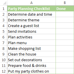
If you are creating an Excel checklist or to-do list, the first step is to make a list of tasks or other items for which the check boxes will be inserted.
For this example, I’ve created the following Party Planning Checklist:
3. Add a check box
The preparation steps are completed, and now we are getting to the main part – add checkboxes to our Party Planning list.
To insert a checkbox in Excel, execute these steps:
- On the Developer tab, in the Controls group, click Insert, and select Check Box under Form Controls.
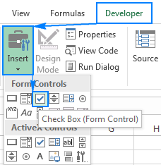
- Click in the cell where you want to insert the first checkbox (B2 in this example). The Check Box control will appear near that place, though not exactly positioned in the cell:
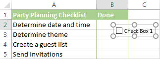
- To properly position the check box, hover your mouse over it and as soon as the cursor changes to a four-pointed arrow, drag the checkbox where you want it.

- To remove the text “Check Box 1“, right click the checkbox, select the text and delete it. Or, right click the check box, select Edit Text in the context menu, and then delete the text.
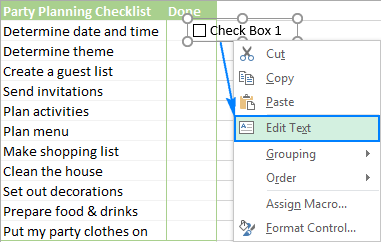
Your first Excel checkbox is ready, and you just have to copy it to other cells.
4. Copy the checkbox to other cells
Select the cell with the check box by using the arrow keys on your keyboard, and position the cursor over the lower right corner of the cell. When the mouse pointer changes to a thin black cross, drag it down to the last cell where you want to copy the checkbox.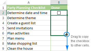
Done! The check boxes are added to all the items in the checklist: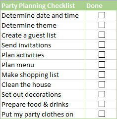
As you can see in the screenshot above, our Excel checklist is almost ready. Why almost? Although the checkboxes are inserted and you can now check or uncheck them by simply clicking on a box, Microsoft Excel is not able to respond to these changes because no cell is linked to any of the checkboxes yet.
The next part of our Excel Checkbox tutorial will teach you how to capture the user selecting or clearing a checkbox and how to use that information in your formulas.
Examples of using checkboxes in Excel
Below you will find a few examples of how to use checkboxes in Excel to make an interactive checklist, to-do list, report and chart. But first, let’s learn how to link checkboxes to cells. The technique is very simple, but it’s the corner stone of using the checkbox results in your formulas.
How to link a checkbox to a cell
As already mentioned, to be able to capture the checkbox state (checked or unchecked) you need to associate the check box with a certain cell. To do this, please follow these steps:
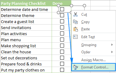
- Right click the checkbox, and then click Format Control.
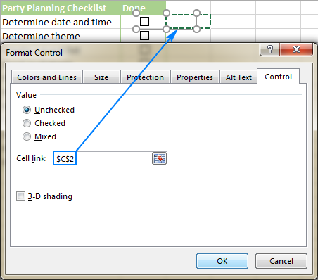
- In the Format Control dialog box, switch to the Control tab, click in the Cell link box and select an empty cell on the sheet to which you want to link to the checkbox, or type the cell reference manually:
- Repeat the above step for other check boxes.Tip. To easily identify the linked cells, select them in an adjacent column that does not contain any other data. This way, you will be able to safely hide the linked cells later so they won’t clutter your worksheet.
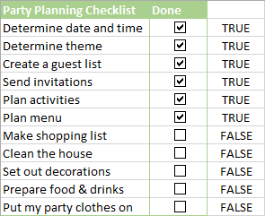
- Finally, click on each of the linked checkboxes. In the linked cells, TRUE appears for selected checkboxes, and FALSE for cleared checkboxes:
At this point, the link cells probably don’t make much sense, but please bear with me just a little longer and you will see how many new opportunities they provide to you.
How to make a checklist in Excel with data summary
In fact, we have already done the major part of the job by adding checkboxes and linking them to cells. Now, we will just write a few formulas to create a data summary for our Excel checklist.
Formula to calculate the total number of tasks
It’s the easiest one – use the COUNTA function to get the number of non-blank cells in the checklist:
=COUNTA(A2:A12)
Where A2:A12 are the checklist items.
Formula to get the number of completed tasks
A completed task means a checkbox with a tick symbol in it, which means the TRUE value in a linked cell. So, get the total count of TRUE’s with this COUNTIF formula:
=COUNTIF(C2:C12,TRUE)
Where C2:C12 are the linked cells.
To make a formula a bit more clever, you use COUNTIFS instead of COUNTIF to check for blank cells in the list (column A):
=COUNTIFS(A2:A12, "<>", C2:C12, TRUE)
In this case, if you delete some irrelevant item(s) from your Excel checklist, but forget to remove a check symbol from the corresponding box, such checkmarks won’t be counted.
Formula to get the percentage of completed tasks
To calculate the presented of the tasks completed, use the regular percentage formula:
Part/Total = Percentage
In our case, divide the number of completed tasks by the total number of tasks, like this:
=COUNTIF(C2:C12,TRUE)/COUNTA(A2:A12)
The following screenshot demonstrates all of the above formulas in action: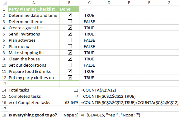
As you can see in the screenshot above, we have inserted one more formula in B18. The formula is based on the IF function that returns “Yes” if the number of completed tasks is equal to the task’s total, “No” otherwise:
=IF(B14=B15, "Yep!", "Nope :(")
To embellish your checklist a bit further, you can create a couple of conditional formatting rules that will change the colour of cell B18 depending on its value.
Once that’s completed, hide the column with linked cells, and your Excel checklist is done!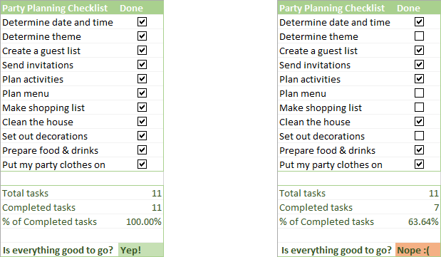
If you like the checklist we’ve created for this example, you are welcome to download it now:
Download this Excel Checklist
More Excel checklist templates
To quickly get a selection of checklist templates for Excel, click File > New, type “checklist” in the search box, and press Enter.
If none of Excel’s checklist templates is well suited for your needs, you may find useful the following resources helpful:
- 50+ printable checklist and to-do list templates (for Excel and Word)
- Free Excel check list templates
- Interactive Excel checklist template (with a number of variations and enhancement)
How to create a To-Do list with conditional formatting
Basically, you can add checkboxes and formulas for a to-do list exactly in the same way as we have just done for the Excel checklist. “What’s the point of writing this section then?” you can ask me. Well, in a typical to-do list, the completed tasks have the strikethrough format like this: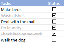
This effect can be easily achieved by creating a conditional formatting rule. The detailed steps follow below.
To begin with, write down a list of tasks, insert checkboxes and link them to cells: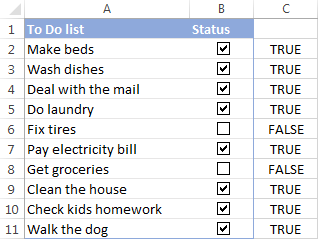
And now, apply conditional formatting that will give the strikethrough format and, optionally, a different background or font color to the checked items.
- Select a list of tasks (A2:A11 in this example).
- Go to the Home tab > Styles group, and click Conditional Formatting > New Rule…
- In the New Formatting Rule dialog box, select Use a formula to determine which cells to format.
- In the Format values where this formula is true box, enter the following formula:
=$C2=TRUEWhere C2 is the top-most linked cell.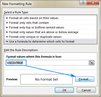
- Click on the Format button, set up the desired formatting style, and click OK. In this example, we select the Strikethrough effect and the light grey font color:
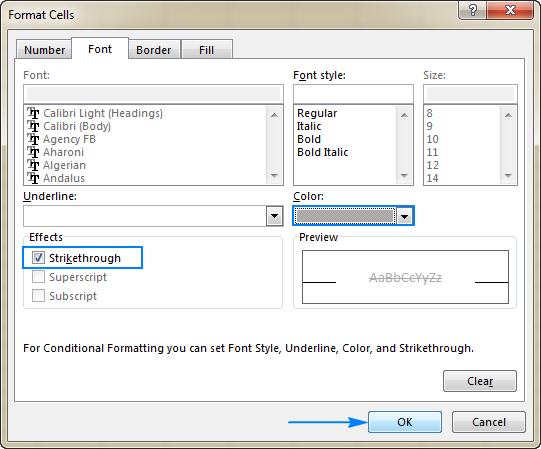 Tip. If you have little experience with conditional formatting, you may find the following detailed guidance helpful: Excel conditional formatting based on another cell value.
As of now, whenever a certain box is checked, the corresponding item gets formatted in the light grey font color with a strikethrough.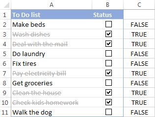
And here’s one more idea for formatting your Excel to-do list. Instead of crossing out the competed tasks, you can insert an additional column with the following IF formula:
=IF(E2=TRUE, "Done", "To Be Done")
Where E2 is the top-most linked cell.
As shown in the screenshot below, the formula returns “Done” if a linked cell contains TRUE, “To be done” if FALSE: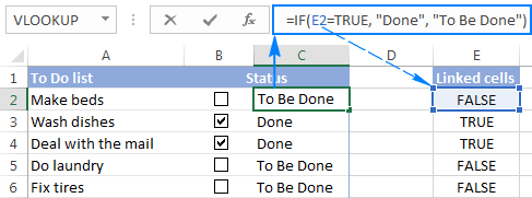
After that, apply the desired conditional format to the Status column based on this formula:
=$C2="Done"
The result will look something similar to this: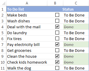
Lastly, add a couple of formulas to calculate the completed tasks (like we did for the checklist), hide the linked cells, and your Excel To Do list is good to go!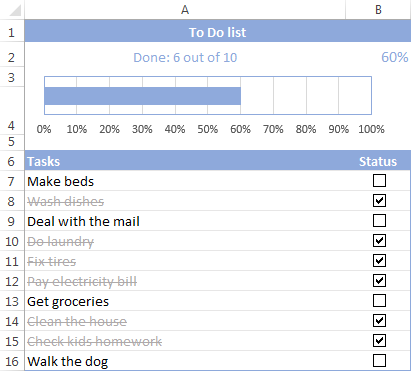
The bar chart at the top of the To-Do list is based on the percentage formula in B2. If you are curious to know the details, I encourage you to download the template, unhide columns D and E, and investigate the formulas.
Download To-Do List Template
How to create an interactive report with check boxes
Another useful application of checkboxes in Excel is for creating interactive reports.
Supposing you have a sales report that includes data for 4 regions: North, South, East and West. Your aim is to get the total for one or more selected regions. Of course, this can be done by using the Slicers feature of an Excel table or PivotTable or by inserting Subtotals. But why don’t we make the report more user-friendly by inserting 4 checkboxes at the top?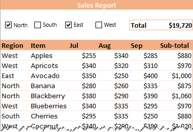
Looks nice, isn’t it? To create a similar report in your sheet, please follow these steps:
- Add 4 checkboxes at the top of the sheet, for the North, South, East and West regions.
- Create the criteria area somewhere in an unused part of the sheet, and link the checkboxes to empty cells:
 In the above screenshot, I2:I5 has linked cells and H2:H5 are the region names exactly as they appear in the report.
 - Add one more column to the criteria area with an IF formula that returns the region name if the linked cell evaluates to TRUE, a dash (“-“) otherwise:
=IF(I2=TRUE, H2, "-")
- Type a heading for the formula column that exactly matches the heading of the corresponding column in the report (Region in this example). The exact match is very important and on the next step, you will understand why.
- Next, write the formula to calculate the total for selected regions. For this, we are going to use the DSUM function that sums the values in a database that match the specified conditions:DSUM(database, field, criteria)Where:
- Database is your table or range including the column headings (A5:F48 in this example).
- Field is the column you want to sum. It can be supplied either as the column heading enclosed in the quotation marks, or a number that represents the position of the column in the database. In this example, we add up numbers in the Sub-total column, so our second argument is “sub-total”.
- Criteria is the range of cells that contain your conditions, including the column heading (J1:J5). That is why the heading of the formula column in the criteria area should match the column heading in the report.Put the above argument together, and your DSUM formula goes as follows:
=DSUM(A5:F48, "sub-total", J1:J5)…and works perfectly!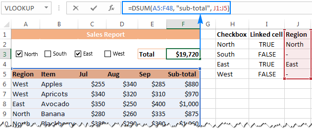
If you’d like to hide the #DIV/0! error that appears when no region is selected, wrap DSUM into the IFERROR function:
=IFERROR(DSUM(A5:F48, "sub-total", J1:J5), 0)
If in addition to total, your report calculates an average for each row, you can use the DAVERAGE(database, field, criteria) function to get a sales average for the selected regions.
Finally, hide and probably lock the criteria area to prevent accidental changes, and your interactive report is all set!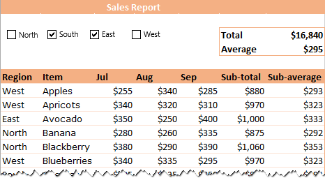
Download Interactive Report
Make a dynamic chart based on the checkbox state
This example will teach you how to create a dynamic Excel chart that can respond to changing the checkboxes state (selected or cleared):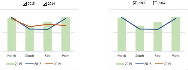
The source data for this example is as simple as this: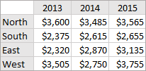
To turn it into a dynamic Excel graph, execute the following steps:
- Create checkboxes and link them to empty cells.In particular, insert 2 checkboxes for the 2013 and 2014 years, and connect them to cells G2 and G3, respectively:
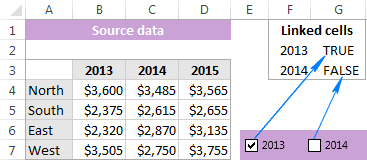
- Create the dataset for the chart dependent on the source data and linked cells (please see the image below):
- For 2013 year (J4:J7), use the following formula:
=IF($G$2=TRUE, B4, NA())If the 2013 checkbox is selected (G2 is TRUE), the formula pulls the original value from B4, otherwise returns the #N/A error. - For 2014 year (K4:K7), enter a similar formula to pull the values from column C if the 2014 checkbox is selected:
=IF($G$2=TRUE, C4, NA()) - In cell L4, enter the formula
=$D4, and copy it down to L7. Because the data for the year 2015 should always be displayed in the chart, an IF formula is not needed for this column.

- For 2013 year (J4:J7), use the following formula:
- Create a combo chart based on the dependent data set (I3:L7). Since we have linked all cells in the dependent table to the original data, the chart will update automatically as soon as any change has been made in the original data set.
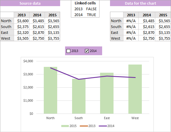
Download Dynamic Chart
This is how you can create and use checkboxes in Excel. To review all the examples discussed in this tutorial, you may want to download our sample workbook below. I thank you for reading and hope to see you on our blog next week.
Ref: https://www.ablebits.com/office-addins-blog/2016/09/21/insert-checkbox-excel/